Training the Decoder#
Now we have a working model with a pre-trained backbone, but we still need to train the decoder. Training this model, however, requires quite a bit of compute and time, if we follow the original training recipe: With a NVIDIA A100 GPU (full-node, 80GB), a batch size of 16 uses almost 90% of the memory and takes around 30 hours to train 12 epochs, on full precision. Training scripts for a SLURM cluster are provided in the scripts/slurm folder, but we’ll first test that everything works correctly.
Testing the Training Script#
To test the training script locally with a single 16GB GPU, can do a couple of things: Reducing batch size, using a smaller model, and enabling mixed precision training:
WANDB_MODE=offline python -m scripts.train_net --num-gpus=1 \
--config-file=projects/dino_dinov2/configs/COCO/dino_dinov2_b_12ep.py \
dataloader.train.total_batch_size=2 \
dataloader.train.num_workers=2 \
train.amp.enabled=True \
model.backbone.net.model_name="vit_small_patch14_dinov2.lvd142m"
In Table 2 we can see how these choices affect both inference speed and memory usage. We should expect mixed precision training to considerably improve over full precision with larger batch sizes, as the former only reduces precision to the activations and not the weights. Furthermore, if the GPU at hand is new enough (Ampere architecture or newer), mixed precision training almost incurs on no accuracy penalty, as it uses the dtype bfloat16.
Backbone |
Precision |
Batch Size |
Time per Iteration |
Memory Usage |
|---|---|---|---|---|
ViT-B |
Full |
2 |
0.8822 s |
11656 MiB |
ViT-B |
Mixed |
2 |
0.6083 s |
9916 MiB |
ViT-S |
Full |
2 |
0.7500 s |
11363 MiB |
ViT-S |
Mixed |
2 |
0.5973 s |
10031 MiB |
Training Setup#
The full training recipe can be found at projects/dino_dinov2/configs/COCO/dino_dinov2_b_12ep.py, which is mostly based on the original recipe for ViT + VitDet + DINO that can be found at detrex/projects/dino/configs/dino-vitdet/dino_vitdet_base_4scale_12ep.py. If you want to create a training recipe for 50 epochs or use a larger dinov2 you can find appropriate recipes in that same folder.
As an example, we can check the optimizer and learning rate scheduler configuration for our recipe.
Show code cell content
import detectron2
from detectron2.config import LazyConfig, instantiate, LazyCall
from omegaconf import OmegaConf
cfg = LazyConfig.load("projects/dino_dinov2/configs/COCO/dino_dinov2_b_12ep.py")
print(OmegaConf.to_yaml(cfg["optimizer"]))
print(OmegaConf.to_yaml(cfg["lr_multiplier"]["scheduler"]))
Thus we can observe that this model is trained with AdamW, with a constant learning rate of 1e-4 for the first 11 epochs, and then decays to 1e-5 for the last epoch, where each epoch is 7500 steps.
The final training command is thus:
python -m scripts.train_net \
--config-file=projects/dino_dinov2/configs/COCO/dino_dinov2_b_12ep.py \
--num-gpus=4 \
train.amp.enabled=False
You can activate automatic mixed precision training by setting train.amp.enabled=True.
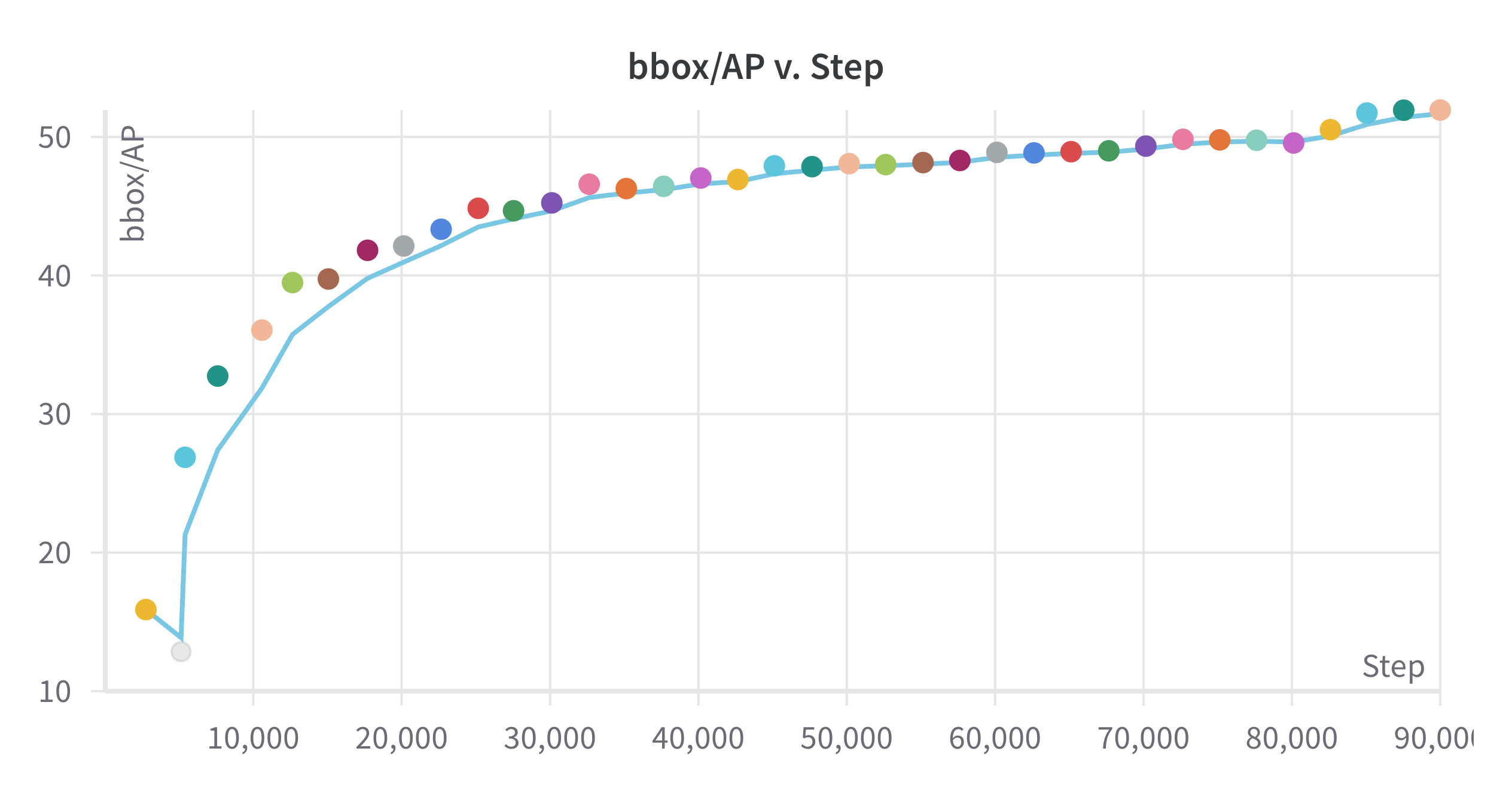
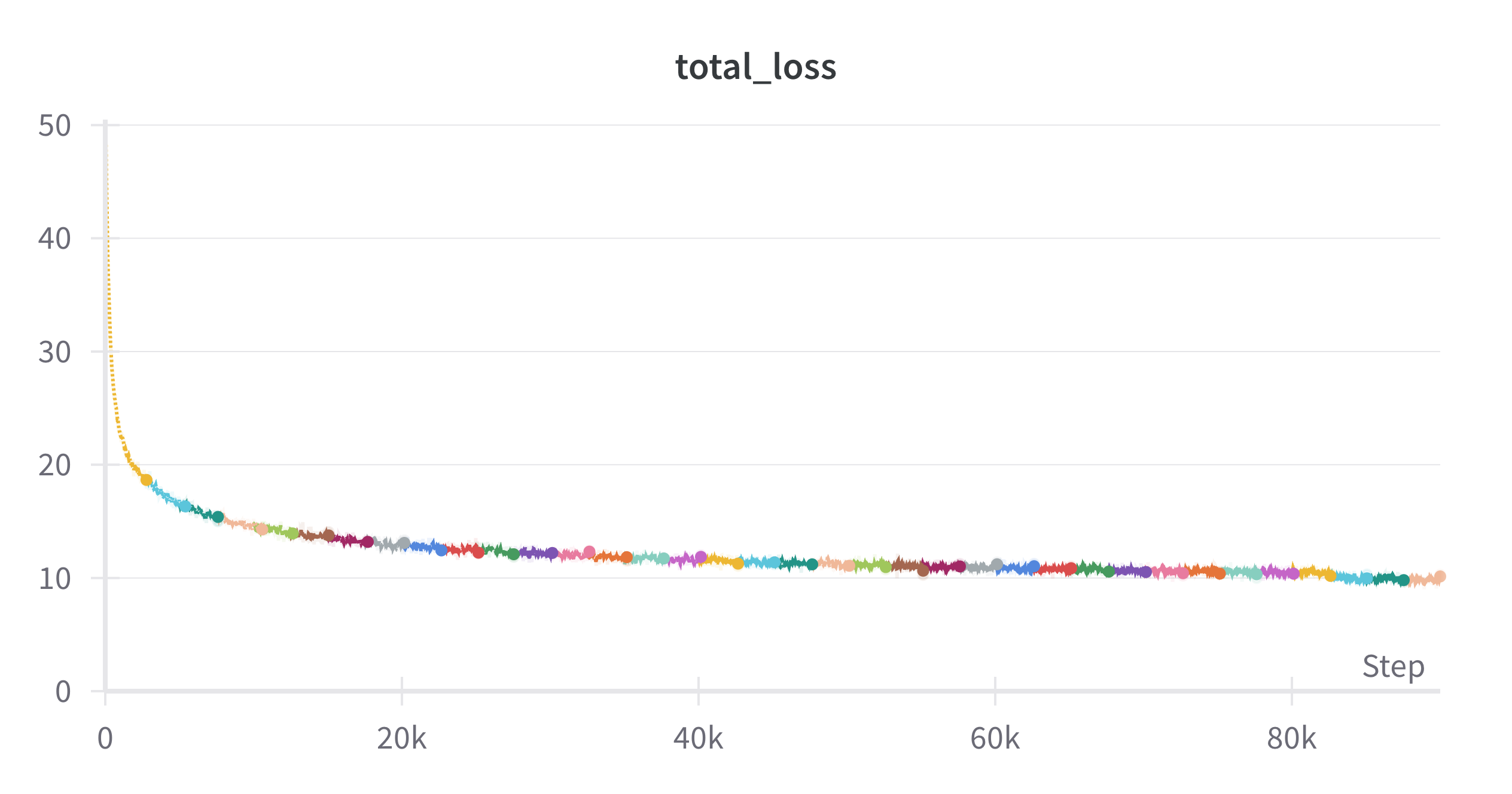
Training Results#
In figures Fig. 9 and Fig. 10 we can see the validation BoxAP and training loss over 12 epochs, respectively. We can observe the little bump in accuracy at the last epoch of training, which is due to the lower learning rate. The model is not saturated, as we can see that the loss is still decreasing.
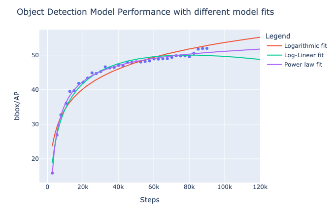
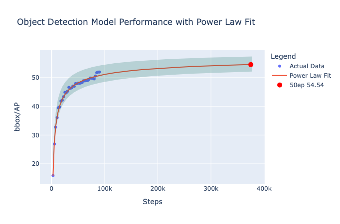
Predicting performance at 50 epochs#
The original model was trained for 50 epochs, so doing a comparison at this stage is unfair. However, we can fit some curves and forecast the performance at 50 epochs. As we can see in Fig. 11, our model’s validation BoxAP is well predicted with a power law. If we extrapolate this curve (see Fig. 12), we can expect a performance of 54.54 at 50 epochs. However, this doesn’t account for the bump in accuracy caused by the learning rate decay, so we can expect a slightly higher performance (~56 AP). 55 box AP is +4.8 points over the original model [LMGH22], which is already a significant improvement.